Mathematical understanding of SPECT data
Single-photon emission computed tomography (SPECT) data is inherently stochastic. It’s stochastic nature comes from the nuclear decay of radioisotopes in the molecular structure of the radiopharmaceuticals.
Mathematical modelling of the “acquisition”
Many and most of the problems in SPECT imaging comes from the following formula of the inverse problem as an operator equation \[ F(u) = g^{\dagger}, \] where the unknown quantity of interest is \(u\), which can be described as an element in a real Banach-space \(X\), the data \(g^{\dagger}\) is non-negative, integrable function on some compact manifold \(\mathbb{M} \subset \mathbb{R}^{d}\) and the possibly non-linear forward operator \(F\) describes the imaging setup.
In general the ideal photon detection can be described by a Poisson point process (PPP) \(G\), the density of which is the marginal spatial photon density \(g^{\dagger}\). Let \(\{x_{1}, \dots, x_{N}\} \subset \mathbb{M}\) denote the positions, where the photons were detected. The total number \(N\) of detected photons is also random. Let \[G = \sum_{i=1}^{N} \delta_{x_{i}}\] as a sum of Dirac-measures at the photon positions and denote by \[G(A)= \#\{1 \leq i \leq N | x_{i} \in A \}\] the number of photons in a measurable subset \(A \subset \mathbb{M}\). Then it is physically evident that \[{\bf E}[G(A)] = \int_{A} g^{\dagger} dx\] and that the random variables \(G(A_{i}), i\in [1, M]\) for any finite number of disjoint, measurable sets \(A_{i} \subset \mathbb{M}\) are stochastically independent. Hence, by definition, \(G\) is a Poisson process, and as a consequence, \(G(A)\) is a poisson distributed integer-valued random variable.
Poisson processes of SPECT data
A point process on \(\mathbb{M}\) can be seen as a random collection of points \(\{ x_{i}, \dots, x_{N} \} \subset \mathbb{M}\) satisfying certain measurability properties.
Definition (Poisson point process)
Let \(g^{\dagger} \in \mathbf{L}^{1}(\mathbb{M})\) with \(g^{\dagger} \geq 0\). A point process \(G = \sum_{i=1}^{N} \delta_{x_{i}}\) is called a Poisson point process (PPP) or Poisson process (PP) with intensity \(g^{\dagger}\) if
For each choice of disjoint, measurable sets \(A_{1}, \dots, A_{n} \subset \mathbb{M}\) random variables \(G(A_{j})\) are stochastically independent.
\({\bf E}[G(A)] = \int_{A} g^{\dagger} dx\) for each measurable set \(A \subset \mathbb{M}\).
Proposition
Let \(G\) be a Poisson process with intensity \(g^{\dagger} \in \mathbf{L}^{1}(\mathbb{M})\). Then for each measurable \(A \subset \mathbb{M}\) the random variable \(G(A)\) is Poisson distributed with parameter \(\lambda = \int_{A} g^{\dagger} dx\), i.e. \({\bf P}[G(A) = k] = e^{-\lambda} \frac{\lambda^{k}}{k!}\) for \(k \in \mathbb{N}\).
Proposition
Poisson process \(G\) with intensity \(g^{\dagger} \in \mathbf{L}^{1}(\mathbb{M})\) conditioned on \(G(\mathbb{M}) = N\) is a Bernoulli process with parameter \(N\) and probability measure \(\mu(A) = \int_{A} g^{\dagger} / \int_{\mathbb{M}}g^{\dagger}dx.\) In other words, conditioned on \(G(\mathbb{M}) = N\) the points are distributed like independent random variables \(X_{1}, \dots, X_{N}\) distributed according to \(\mu\).
Poisson process characteristics
Few of the properties of the Poisson processes are the following
Lawfulness
It means that the events are not arriving in the exact same time \[\lim_{\Delta t \rightarrow 0} P(G(t + \Delta t) - G(t) > 1\ |\ G(t + \Delta t) - G(t) \geq 1 ) = 0\]
Memory-less, ageless
This means that the events arriving after another are stochastically independent. \[P(G(A) > a + b\ |\ G(A) > a) = P(G(A) > b) \]
Zleho ideas, Markov processes
Sensitivity is a constant multiplier on the pixel values
Pixel values are independent, isotropically independent, binning is independent
They are independent as much as phone calls, it is like histogramming the areas and centers
Gaussian approximation will be good with a weighted least squares, division by stdev will result in a good approximation
Photon decay, between two decay time is exponential, linear transform of poisson will be our image
Projection data of SPECT
Approximation in L2
Approximating the original frames in \(\mathbb{L}_{2}\)
L2 approximation error (sum): 0.0001685299889809691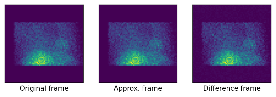
prof_orig_proj = proj_data_par[0, 32, :]
prof_appr_proj = appr_proj[32, :]
prof_appr_std_dev_proj = appr_std_dev_proj[32, :]
prof_diff_proj = diff_orig_appr_proj[32, :]

x = np.arange(0, 64, 1)

fig, ax = plt.subplots()

ax.plot(x, prof_diff_proj)
#ax.plot(x, prof_appr_std_dev_proj)
ax.set_xlabel("Profile curve of the difference")
Text(0.5, 0, 'Profile curve of the difference')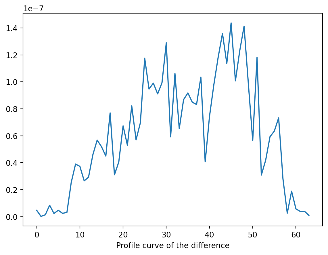
print(np.std(proj_data_par[0]))12.85805956206453